StreamflowPyML
 Photo by Gianluca Bei on Unsplash
Motivation and Background
This project was completed as a component of the Part Time Data Science Course through BrainStation completed in Spring 2020. Prior to the course I had been working in R to build interactive applications in Shiny and I took the BrainStation data science course to get familiar with Python prior to starting a Master of Data Science (MDS) degree at UBC.
The purpose of the study was to assess the ability to use machine learning to estimate daily streamflow in British Columbia (BC), Canada using streamflow and climate data in proximity to a stream of interest. The study was considered an initial step in determining if an automated or semi-automated procedure could be applied to generate machine learning models for any streamflow location in British Columbia. The modelling completed in this study is certainly outdated by the level of information from the MDS program but it was an interesting exercise for both learning python and applying machine learning models to a non-standard dataset.
The work was completed in Jupyter Notebook and can be viewed in html and the supporting datasets and code are available in github.
Study
A detailed discussion of the study is available in the Jupyter Notebook and this overview aims to provide a brief summary of the analysis.
Dataset
Stave River streamflow data was selected for the study due to previous experience with the data.
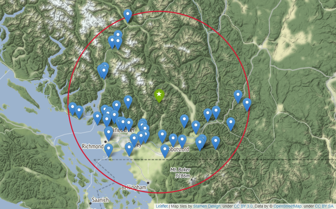
R was used to download the streamflow and climate data in the vicinity of the Stave River using the tidyhydat and weathercan packages. This was done as these R packages are well maintained and have been built to access Water Survey of Canada (WSC) and Environment and Climate Change Canada (ECCC) databases. The hydrometric and climate stations within a 100 km radius from the Stave River are shown in the figure below.
The compiled dataset included 98 features of temperature, precipitation, and streamflow from surrounding hydrometric and climate stations with daily data from 1983 to 2016. The following steps were taken to clean the dataset:
- Due to the high number of features, any stations with greater than 10% of missing data was removed resulting in a remaining set of 63 features.
- Missing data were infilled using the monthly mean.
- For each of the remaining 63 features, additional features were added corresponding to previous 1-day and previous 7-day mean values. This was done as streamflow can be very dependent on forcings prior to the given date due to a lag time effect.
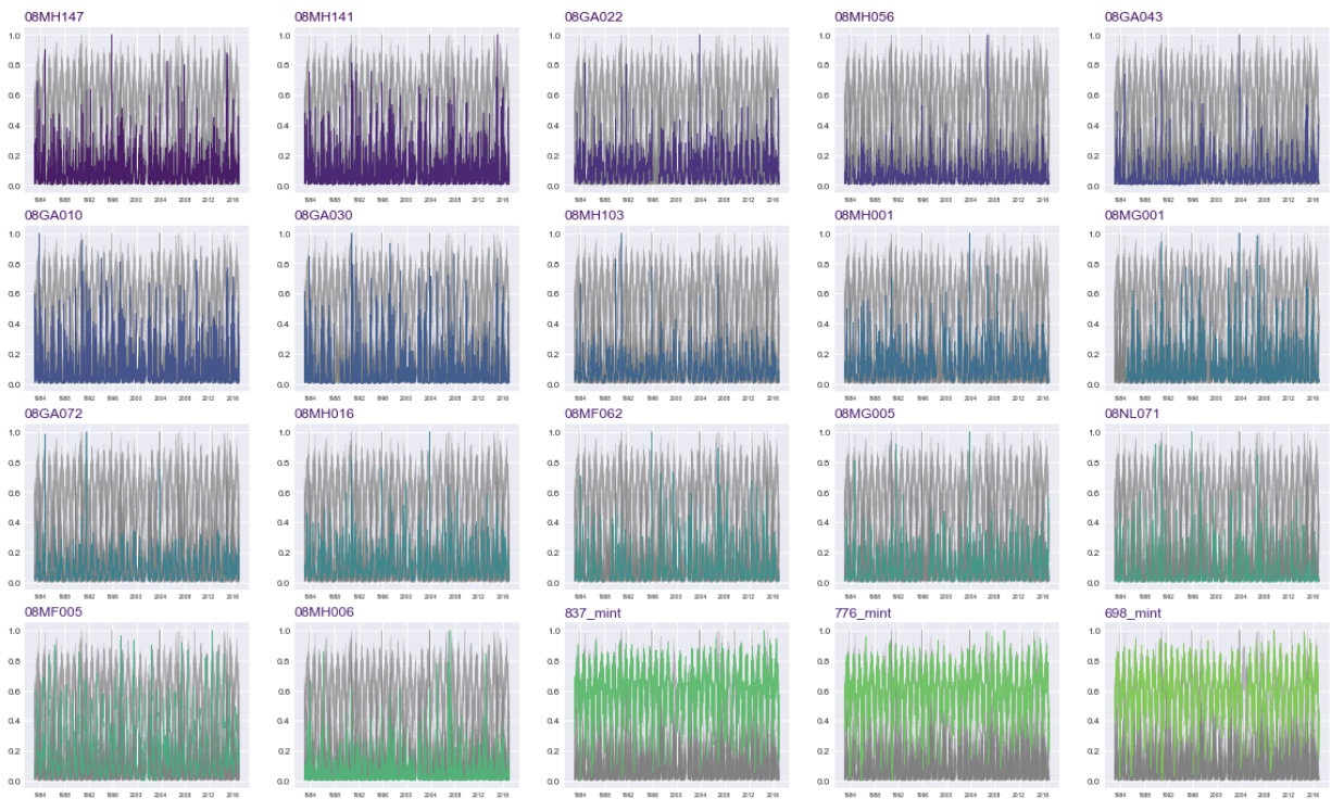
A normalized timeseries review of the top 20 correlated features with the Stave River streamflow was looked at to understand the general pattern of the data. Each subplot in the figure below highlights a single feature overlaid on all of the normalized data (shown in grey) in an attempt to understand the pattern of each feature with respect to other data. Most of the features follow a similar pattern but it can be observed that some experience more extreme peak values whereas others are more uniform. The hope was that these features would provide sufficient variety of data to model the Stave River streamflow over the full range of flow conditions.
Modelling
Modelling was completed using Scikit-learn and three models were used in the analysis:
- Linear regression using ordinary least squares
- Random forest regression
- Gradient boosting regression
A 75% training and 25% testing set split was used to assess/compare the model results. Feature reduction was also used as follows:
- Recursive feature selection and cross-validation (RFECV): using the built-in Scikit-learn function to auto-reduce features in the linear regression model to the optimal number generated from the procedure.
- Feature Importance: any features with an importance of < 1% for the random forest and gradient boosting models were dropped. While this is somewhat arbitrary and it may certainly be possible to use a higher threshold, the purpose of the study is to asses an automatable or semi-automatable approach so the selection of a standard threshold was used.
Note that for the Random Forest and Gradient Boosting model, no hyperparameters were tuned. Accordingly, it is expected that better performance could be gained for these model.
Comparison of Results
Each of these three models were applied to the datasets both including and excluding the previous 1-day and previous 7-day mean values. A comparison of metrics for the models are provided in the table below.
| Model | Metric | Train excl prev | Test excl prev | Train incl prev | Test incl prev |
|---|---|---|---|---|---|
| Linear | RMSE | 9.328 | 9.379 | 8.551 | 9.133 |
| Linear | $R^2$ | 0.932 | 0.923 | 0.942 | 0.928 |
| Random Forest | RMSE | 3.635 | 10.070 | 3.728 | 9.741 |
| Random Forest | $R^2$ | 0.990 | 0.912 | 0.989 | 0.918 |
| Gradient Boost | RMSE | 7.243 | 9.788 | 6.968 | 9.479 |
| Gradient Boost | $R^2$ | 0.959 | 0.916 | 0.962 | 0.922 |
The comparison of results indicates the following:
- The three model types have similar performance. The linear model has slightly better performance but the difference between the three model types is minimal.
- There is overfitting for both the random forest and gradient boosting models, but the testing performance is still similar to the linear regression model.
- There is slightly better performance in metrics for the models that use the previous values dataset in comparison with the models that do not. Therefore, it is considered worth using the previous value features in modelling.
Due to the similarity in model results, a comparison of the 0.1 increment quantiles of observed and modelled Stave River streamflow was also completed as presented in the following figure. Most of the results are similar but the first 0.1 increment quantile (representing low/base flows) indicates that the linear model (blue line) has an overestimation bias and the gradient boosting model (green line) has an underestimation bias. Accordingly, the random forest model (orange line) likely represents the best model from the exercise.

Conclusion
The models were able to provide a reasonable fit for streamflow at Stave River and the exercise indicates that using an automated or semi-automated approach to estimate streamflow at stations in British Columbia may be feasible. The random forest model appeared to outperform linear regression and gradient boosting but hyperparameter tuning was not considered and the results are generally similar.
Summary
This initial study provides a good first step towards utilizing machine learning models for streamflow in British Columbia but additional study should be considered including assessing:
- Locations within different regions of the province.
- Models utilizing sparser regionally available datasets.
- The impact in the reduction of data record length (minimum length of record required by the model to perform adequately).
- Review of other machine learning models and/or the tuning of model parameters (defaults were used in this study).
- Comparison of accuracy with existing methods such as Empirical Frequency Pairing.
This project was primarily motivated by learning Python and starting to apply machine learning models to non-standard datasets. The project goals were achieved based on this learning objective but it would be interesting to consider the items above for a future side-project.
Nathan Smith
Data Scientist
Solving problems using data science coupled with a background in water resource engineering.